Effect of Sunlight on the Biodiversity of Soil Invertebrates

Loretta McNamee

Undergraduate Student

(Environmental Biology Concentration), Department of Biology, Tennessee Tech University , Cookeville, TN 38505

 -------------------------------------------------------------------------------------------------------------------------------------------------------------

Abstract:

EFFECT OF SUNLIGHT ON THE BIODIVERSITY OF SOIL INVERTEBRATES

Loretta A. McNamee

 (Environmental Biology Concentration), Department of Biology, Tennessee Tech University, Cookeville, Tennessee  38505

The purpose of this research project was to determine if sunlight affects the soil biodiversity of soil invertebrate. By using two distinct communities, canopy and open ground, examination of the purpose was possible. The null hypothesis states that there is no difference in the two communities. Eight samples from each habitat were collected (16 total). Each sample was then put into a berlese funnel system and organisms were collected after a week. Organisms were identified and counted according to species. Multiple statistical tests were performed on the data including two population t-tests and the Kolmogorov-Smirnov test. Species richness, species diversity, and species evenness were all used to determine species diversity. These biodiversity measurements included the Simpson and Shannon Indexes. Species accumulation and rank-abundance curves were created to help illustrate the data found. The results showed that there was no difference between the two distinct communities. However, it did show that the canopy habitat had more species evenness than the open ground habitat. Also the null hypothesis was indeed accepted due to the fact that t-stat was less than t-critical values. There are many reasons why this occurred such as; the presence of intraspecific competition between the different species found, or presence of alder on top of soil. This research gives new perspective towards older studies that say that there are differences in the communities.

 -------------------------------------------------------------------------------------------------------------------------------------------------------------

Key Words

Here is a list of key words that will help identify the experiment when put into a search engine:

Soil

Biodiversity

Collembola

Species richness

Invertebrate

Hymenoptera

Annelid

Species Accumulation curve

Ecosystem

Mutualistic relationship

Terrestrial

Carbon

Decomposition

Abundance

Intraspecific competition

 -------------------------------------------------------------------------------------------------------------------------------------------------------------

Introduction

Soil biodiversity is the number and abundance of species inhabiting a community or a habitat. It is a very important starting point to explaining patterns of community dynamics and structure. However, this huge community is often unnoticed by most people, but it plays such a vital role in the soil community dynamics. The invertebrate influence many soil properties (water levels, carbon levels, and nutrient levels), which influence above-ground plant abundance. The objective of this experiment is to examine soil biodiversity in soil invertebrates in two distinct communities; canopy and open ground. Also the null hypothesis states there will be no difference in the communities.

One study showed that many chemical and physical properties of the soil differ based on its location (Pankhurst 1992).  These chemical and physical properties influence what type of organisms can survive in that type of soil. The amount of moisture or the amount of carbon would affect such property (Briones 2006). Other studies suggest that the presence of plants (alder) affects the communities in the soil (Dunfield 2003, Chamberlain 2006). The Dunfield study also suggests that plants provide nutrients that the soil organisms can utilize for survival. However, the Chamberlain study suggests that the reason for a high abundance of Collembola is the large presence of alder.  If these studies are correct the forest or canopy environment of the biodiversity experiment should have more invertebrates present. Another study done by Ferguson, stated that soil invertebrate would rather be under soil that is covered, no matter if it was natural or artificial (2004). This would coincide with my hypothesis that stated the canopy habitat would have a greater soil biodiversity.

------------------------------------------------------------------------------------------------------------------------------------------------------------- 

Methods and Materials:

Soil invertebrate communities were examined by the use of two distinct habitats to show the biodiversity of the soil invertebrates. The habitats were located on the campus of Tennessee Tech University in the area at the back of the varsity baseball field. An open ground habitat and a forest (canopy) habitat were chosen in order to have two completely different habitats. Sixteen plastic bags (eight for each habitat) and a garden tool were used to collect the samples. Once at each habitat, a soil sample was taken from eight different spots around each habitat and placed into separate plastic bags.

            Once the samples were obtained, they were taken to the laboratory to set up a Berlese funnel.  In order to create a funnel system for each habitat a mason jar, funnel, light bulb, alcohol, and a mesh screen were all needed. The mesh screen was put at the bottom of the funnel and then the funnel was placed in the top of the mason jar (that had alcohol in the bottom). A soil sample from the forest habitat was put into the funnel and kept under a light bulb to ensure it dried out the soil. The exact same set-up was used for the rest of the forest habitat and all of the open ground habitat. So in total there were sixteen burlese funnels set up around the lab.

            The samples were left to dry for a week. After the week the mason jars with the invertebrates at the bottom were obtained from the lab. Each Jar’s content was filtered to gather the organisms. This was done by placing filter paper in the funnel and pouring the alcohol and organisms in the funnel, steps were repeated until all the organisms were out of the jar and nicely on the filter paper. Once all the organisms were filtered out, they were put under the microscope. Once there, they were identified into different species (using identity sheet) and then counted by species.

            Once all the data was obtained, a number of  various statistical tests were performed on the data to help come to a conclusion. For each habitat, the species richness, species Diversity (H and D), and species evenness (J and E) were all found.  A species accumulation curve and a rank-abundance curve were created using the data. Two methods of statistical analysis were used to compare the habitats to see if they differ, they were; the t-tests and the Kolmogorov-Smirnov test.

Citations for statistical tests and methods:

2006, William M.K. Trochim, http://www.socialresearchmethods.net/kb/stat_t.php

College of saint benedict. http://www.physics.csbsju.edu/stats/KS-test.html  

For methods: Dr. Chris Brown, 2007

-------------------------------------------------------------------------------------------------------------------------------------------------------------

Results:

The data that was collected during the experiment is shown in tables 1 and 2. These tables illustrate the entire experiment’s data and show how each individual was collected through sample numbers. Tables 3 and 4 show more depth information of the data, this gives the necessary data needed to calculate the tests done on the two habitats. Tables 3 and 4, give the statistical data gathered from the sampling that is used to calculate the measures of biodiversity.  In table 5, the final calculations of biodiversity measurements are found for each community.

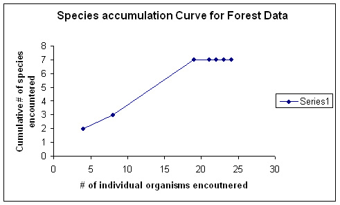
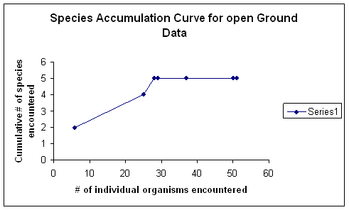
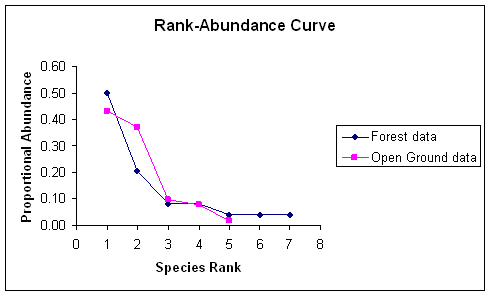
            Figures 1 and 2 shows the species accumulation curve for both habitats. These curves are the Cumulative number of species encountered vs. the number of individual organisms encountered. Figure 3 illustrates the rank-abundance curve for both habitats, which is the proportional abundance versus species rank. All the values of the Shannon Index for both habitats were put into table 6. The data from table 6 was then put into a two population t-test, which is shown in table 7. The information needed to perform the kolmogorov- Smirnov test, which gives the pi cumulative data is all found in table 8.

Table 1:

Forest (canopy) Data

Table 2:

Open Ground Data

Table 3: Forest Data table

Table 4: Open ground data

Table 5: Biodiversity Measures for Both Habitats

Figure 1:

Figure 2:

Figure 3:

Table 6:

Shannon Index Data

Table 7:

Table 8: Kolmogorov-Smirnov (K-S) Test Data

-------------------------------------------------------------------------------------------------------------------------------------------------------------

Discussion:

            After performing the experiment and analyzing all of the data, it was concluded that there was no difference in the two distinct habitats; forest and open ground. This does contradict the original hypothesis that stated that there would be a distinct difference in the two habitats. A conclusion was met by performing statistical tests and produced graphs of the data collected.

            The graphical information was very important because it supported the findings. Figures 1 and 2 show that it takes more individuals to increase species size in the open ground data than in the forest data. This is important because this is why there was such a higher abundance of invertebrate found in the open ground habitat. Then there is figure 3, which illustrates the rank-abundance curve for both habitats. This graph shows that the forest data is less even then open ground data due to the steep slope on the graph. However, the difference is so small that it is insignificant and doesn’t affect the overall conclusion of the experiment.

During the Kolmogorov-Smirnov, it was found that Dmax was less than Dcrit. According to this, D_crit is greater than D_max,  therefore, the two (field and forest/canopy) communities do not differ in species diversity. The t-test supported the K-S result because it accepted the null hypothesis that stated that there was no difference in biodiversity between the two habitats. All the other information that was gathered supports this conclusion; it also gave us insight that even though there is no difference in diversity the forest data showed more evenness than the open ground data. This was concluded using the measurements of H, D, E, and J. For example, the forest data’s H and D were larger than the open ground’s data H and D, but only by a small amount. The small amount might account for the fact that the forest data has a slightly higher diversity than the ground data.

Although the results show that the two distinct communities showed no difference in species diversity, most previous long term studies show a great difference. A study done by Ferguson, stated that soil invertebrate would rather be under soil that is covered, no matter if it was natural or artificial (2004). This would have coincided with my hypothesis that stated the canopy habitat would have a greater soil biodiversity if the results supported it. Another study showed that many chemical and physical properties of the soil differ based on its location (Pankhurst 1992).  These chemical and physical properties influence what type of organisms can survive in that type of soil. The amount of moisture or the amount of carbon would affect such property (Brione 2006). Other studies suggest that the presence of plants (alder) affects the communities in the soil (Dunfield 2003, Chamberlain 2006). The Dunfield study suggests that the plants provide nutrients that the soil organisms can use for survival. While the Chamberlain study suggests that a large presence of alder is the reason for a high abundance of Collembola.  If these studies are correct the forest or canopy environment of the biodiversity experiment should have had more invertebrates present. A bigger sample size and more distinct habitats would have helped the experiment be more accurate. However, this experiment did produce good results and had a definite conclusion.

-------------------------------------------------------------------------------------------------------------------------------------------------------------

Conclusion:

      No difference was found in soil invertebrate biodiversity between the two distinct

habitats. The null hypothesis was accepted, and the hypothesis that stated the canopy community would have greater soil biodiversity was rejected. Forest Data was found to be less even than open ground, but had more abundance of species. That data was collected through the evaluations of the species diversity measurements.  Both Kolmogorov-Smirnov and t-tests statistically showed no difference between the two distinct communities.

Acknowledgments:

            I would like to thank Dr. Brown for being able to utilize his methods for this experiment. I would also like to thank Emily Shrum for her help in collecting samples and setting up the Berlese funnels in the laboratory.

-------------------------------------------------------------------------------------------------------------------------------------------------------------

Works Cited

Briones, M.J.,Ostle N.J., Garnett M.H. 2006. Invertebrates increase the sensitivity of non-

            labile soil carbon to Climate Change. Soil Biology & Biochemistry 39(3): 816-818

Chamberlain, P.M., and McNamara, N.P.2006 Translocation of Surface litter Carbon into

            Soil by Collembola. Soil Biology & Biochemistry. 9:2655-2664.

Dunfield, K.E., and Germida, J.J. 2003. Impact of Genetically Modified Crops on Soil

and Plant Associated Microbial Communities.  Journal of Environmental Quality. 

33:799-804.

Ferguson, S.H., and Berube, D.K. Invertebrate Diversity under Artificial cover in

Relation to Boreal Forest Habitat Characteristics. Canadian Field-Naturalist.3:

386-394.

Heemsbergen, D.A., Berg, M.P., Loreau, M., van Hal,J.R..2004.Biodiversity effects on

soil processes explained by Interspecific functional dissimilarity. (Reports). Science 306: 1019-1021. 

-------------------------------------------------------------------------------------------------------------------------------------------------------------

Appendix:

Effect of sunlight on biodiversity of soil invertebrates

Location: __________________________________________________________________

                    (Facility name)                                 (City)                (County)          (State)   

Sample Taken by: ___________________________________________________________

                                (Name)                     (Position)                    (Organization)

___________________________________________________________________

Table 1: Forest (canopy) Data

Table 2: Open Ground Data

Table 3: Forest Data table

Table 4: open ground data